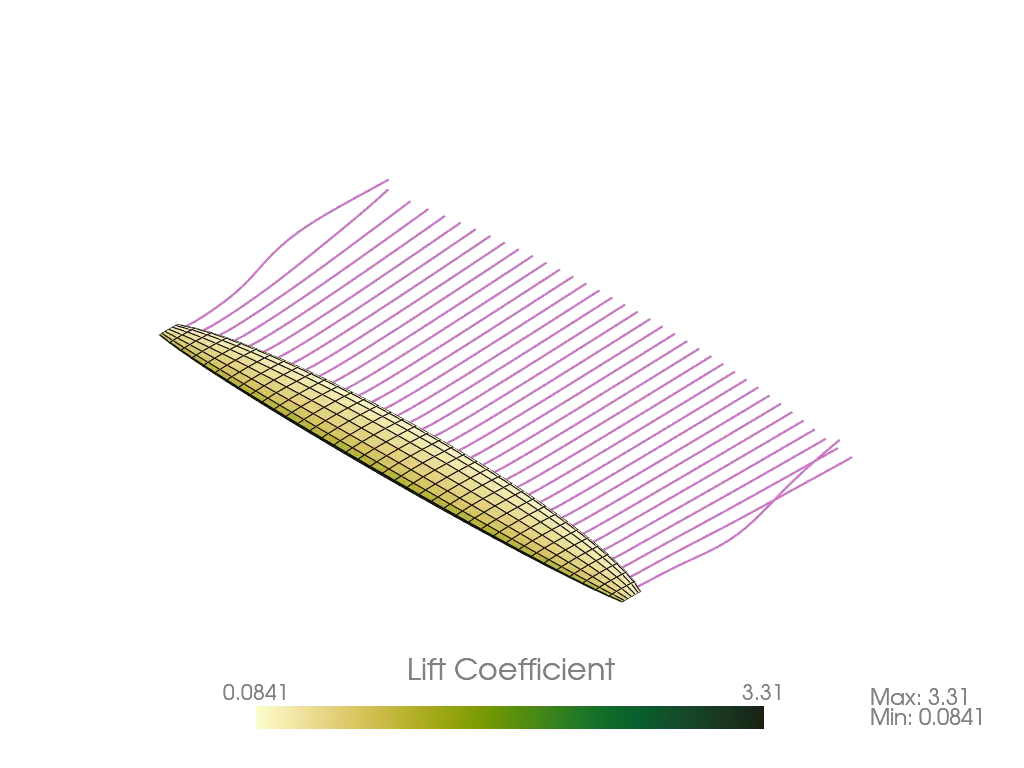
"""Demonstrates running Ptera Software's SteadyRingVortexLatticeMethodSolver on a non-
trapezoidal Wing built from leading and trailing edge curves.

Instead of describing a Wing by its trapezoidal WingCrossSection corners, this example
builds an elliptical planform, the classic non-trapezoidal wing shape, directly from
samples of its leading and trailing edge curves with Wing.from_edge_points.

The script will log simulation results in a log file.
"""

import logging

# NumPy is used here only to build the edge curves. It is not required to use Ptera
# Software in general.
import numpy as np

# First, import the software's main package. Note that if you wished to import this
# software into another package, you would first install it by running "pip install
# pterasoftware" in your terminal.
import pterasoftware as ps

# Configure logging to write info level messages to a file. To display log messages on
# the console alongside progress bars instead, omit the handler argument.
ps.set_up_logging(level="Info", handler=logging.FileHandler("example_solver.log"))

# Sample the leading and trailing edge curves of an elliptical planform. The curves are
# expressed in wing axes, relative to the leading edge root point, in meters. We sample
# them densely here. from_edge_points resamples both curves to the requested number of
# WingCrossSections, so this input resolution is independent of the final mesh.
root_chord = 1.5
span = 6.0
num_edge_samples = 100
ys_Wn_Ler = np.linspace(0.0, span, num_edge_samples)

# An elliptical chord distribution tapers smoothly from the root chord to a point at the
# tip.
chords = root_chord * np.sqrt(1.0 - (ys_Wn_Ler / span) ** 2)

# Keep the quarter chord line straight along the span, which is what makes the planform
# a true ellipse. The leading edge and trailing edge then follow from the quarter chord
# position and the local chord. The leading edge starts at the origin (the leading edge
# root point) and the trailing edge starts at the root chord, as from_edge_points
# requires.
quarter_chord_x = root_chord / 4.0
leading_edge_xs = quarter_chord_x - 0.25 * chords
trailing_edge_xs = quarter_chord_x + 0.75 * chords

# Assemble the (M, 3) edge point arrays. from_edge_points builds planar Wings, so every
# z component is zero.
zeros = np.zeros_like(ys_Wn_Ler)
leadingEdgePoints_Wn_Ler = np.column_stack((leading_edge_xs, ys_Wn_Ler, zeros))
trailingEdgePoints_Wn_Ler = np.column_stack((trailing_edge_xs, ys_Wn_Ler, zeros))

# Create an Airplane with our custom geometry. As in the other examples, I am going to
# declare every parameter even though most of them have usable default values. This is
# for educational purposes, but keep in mind that it makes the code much longer than it
# needs to be. For details about each parameter, read the detailed class and method
# docstrings.
example_airplane = ps.geometry.airplane.Airplane(
    wings=[
        # Build the Wing from its edge curves rather than from trapezoidal
        # WingCrossSection corners. from_edge_points resamples the curves into a
        # sequence of single-panel strips that approximate the elliptical planform. An
        # elliptical planform tapers to a point at the tip, where the chord would be
        # zero, so we use tip_trim_fraction to drop a small fraction of the span off the
        # tip and leave the outermost WingCrossSection with a finite chord.
        ps.geometry.wing.Wing.from_edge_points(
            leadingEdgePoints_Wn_Ler=leadingEdgePoints_Wn_Ler,
            trailingEdgePoints_Wn_Ler=trailingEdgePoints_Wn_Ler,
            num_wing_cross_sections=20,
            airfoil=ps.geometry.airfoil.Airfoil(
                name="naca2412",
                outline_A_lp=None,
                resample=True,
                n_points_per_side=400,
            ),
            name="Main Wing",
            Ler_Gs_Cgs=(0.0, 0.0, 0.0),
            angles_Gs_to_Wn_ixyz=(0.0, 0.0, 0.0),
            symmetric=True,
            mirror_only=False,
            symmetryNormal_G=(0.0, 1.0, 0.0),
            symmetryPoint_G_Cg=(0.0, 0.0, 0.0),
            num_chordwise_panels=8,
            chordwise_spacing="cosine",
            tip_trim_fraction=0.05,
        ),
    ],
    name="Example Airplane",
    Cg_GP1_CgP1=(0.0, 0.0, 0.0),
    weight=0.0,
    s_ref=None,
    c_ref=None,
    b_ref=None,
)

# Define a new OperatingPoint, which we'll pass into the SteadyProblem.
example_operating_point = ps.operating_point.OperatingPoint(
    rho=1.225, vCg__E=10.0, alpha=5.0, beta=0.0, externalFX_W=0.0, nu=15.06e-6
)

# Define a new SteadyProblem, which contains the OperatingPoint and a list of one or
# more Airplanes.
example_problem = ps.problems.SteadyProblem(
    airplanes=[example_airplane],
    operating_point=example_operating_point,
)

# Now that the Airplane and OperatingPoints exist within the SteadyProblem, I like to
# delete the external pointers to these objects to ease debugging.
del example_airplane
del example_operating_point

# Define a new solver. The available solver classes are
# SteadyHorseshoeVortexLatticeMethodSolver, SteadyRingVortexLatticeMethodSolver, and
# UnsteadyRingVortexLatticeMethodSolver. We'll create a
# SteadyRingVortexLatticeMethodSolver, which requires a SteadyProblem.
example_solver = (
    ps.steady_ring_vortex_lattice_method.SteadyRingVortexLatticeMethodSolver(
        steady_problem=example_problem
    )
)

del example_problem

# Run the solver.
example_solver.run()

# Save the solved solver to a compressed JSON file. This allows us to load the results
# later without re-running the simulation. Use ".json.gz" for gzip compression, which is
# recommended over plain JSONs for all but the smallest, unmeshed geometry objects.
ps.save("example_solver.json.gz", example_solver)

# Load the saved solver. The loaded object is identical to the original and can be
# passed to any output function.
loaded_solver = ps.load("example_solver.json.gz")

# Call this function from the output module to log the results.
ps.output.log_results(loaded_solver)

# Call the output module's draw function on the loaded solver.
ps.output.draw(
    solver=loaded_solver,
    scalar_type="lift",
    show_streamlines=True,
    show_wake_vortices=False,
    save=True,
    testing=False,
)